In discussing the distribution of faunal remains in my analyzed sample, I will seek to describe the faunal assemblage in a way that is meaningful for understanding human behavior. For this reason, I will reduce the number of analytical groups by lumping taxonomic categories based on methods of capture and processing.
To facilitate the direct comparison of faunal data from excavation units of varying size, I have employed the Volume Control Constant (KV) introduced in Section 3. Multiplying all data from a sample by KV allows me to pretend for analytic purposes that all data derive from uniform excavation units, one square meter in area and 10 cm thick. Such an approach misrepresents the relative taxonomic richness of a sample, which varies as a function of sample size (Grayson 1981:82–83). As the number of individual specimens recovered rises, the number of taxa identified should also rise; by manipulating my data with KV, I prevent the direct comparison of taxonomic richness between samples.
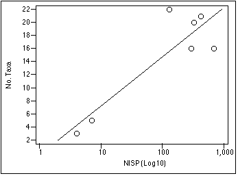
Figure 5.1, correlation of number of individual specimens and number of taxa in a sample. Best fit line is a power function of the form f(x) = a + bxc. NISP reflects numbers of individual specimens, not adjusted for volume.
Figure 5.1 demonstrates the relationship of NISP to taxonomic variation. In general, the number of taxa in a unit will rise exponentially as a function of NISP. The moderate correlation between NISP and number of taxa observed (R2 = 0.775) in this instance is probably due to the small number of sample units (n = 7). If I had identified more individuals to finer taxonomic resolution, then the total numbers of taxa identified would also be higher, possibly providing a stronger correlation between NISP and taxonomic richness.
As with the review of analyzed samples in Section 4, unless otherwise noted, all data referred to in Section 5 were derived from analyses of the 1/4" screen sample. Some data from analyses of bulk soil samples were germane to my discussion, however, and I will note the source of these data when I introduce them.
Distribution of Bird Remains
Remains of cliffdwelling birds—auks and cormorants—are the most abundant type of bird in the total analyzed sample (Figure 5.2) . When adjusted for excavation volume, Alcidae and Phalacrocoracidae represent the most abundant birds by all measures, comprising 58% of the identified bird sample by NISP, 49% by MNI, and 59% by bone weight. The presence of a single large Phalacrocorax individual in the TU7/7 sample may overrepresent cliff birds by weight, although their remains dominate the sample by measures of MNI and NISP as well. Birds usually caught while nesting or on open water—ducks, grebes, and loons—occur roughly as frequently as gulls; these two groups essentially tie for second place in abundance.
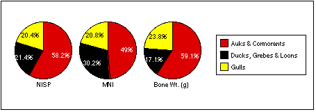
Figure 5.2: Identified bird remains from all analyzed samples, by Number of Individual Specimens, Minimum Number of Individuals, and Bone Weight. All measures adjusted for volume.
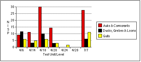
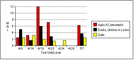
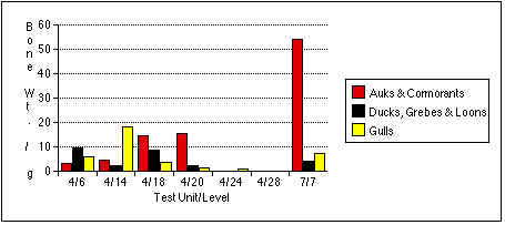
Figure 5.3a–c: Identified bird remains from analyzed samples, by Number of Individual Specimens, Minimum Number of Individuals, and Bone Weight. All measures adjusted for volume.
I noted auk and cormorant remains in all but two analyzed samples. After adjustments for excavated volume, sample units 4/18, 4/20, and 7/7 contain the greatest concentrations of these birds, as indicated by all measures (Figure 5.3a–c) . Cliff bird remains predominate in two other units: 4/6 and 4/14. Only the two levels near the bottom of Test Unit 4 (4/24 and 4/28) produced no Alcidae or Phalacrocoracidae bones. Cliff bird remains also tend to occur in larger concentrations than those of other birds (4/18 and 4/20); these loci may represent areas devoted to processing or dumping auk and cormorant remains.
The remains of marsh birds share a similar distribution to cliff birds, although in generally lower numbers. Only sample 4/6 produced the remains of ducks, grebes, and loons in greater relative quantity than those of auks and cormorants by all measures.
Larid remains are the most widely dispersed of all bird types, but often occur in the lowest numbers. Gull remains are the most abundant by NISP in sample 7/7, but more abundant by MNI and bone weight in sample 4/14. Larid bones occur in roughly equal frequencies throughout the other samples; they are the only birds identified in the Stratum IV soils from Test Unit 4.
Distribution of Fish Remains
Gadus macrocephalus distantly outrank all other identified fish taxa in the 1/4" screen sample (Figure 5.4). Pacific cod comprise 90.1% of NISP, 68.5% of the MNI, and 95.5% of the total weight of identified fish bone. With an analyzed piscine sample so overwhelmingly monopolized by a single species, I have difficultly addressing the relative importance of other species, except to note that Nash Harbor people also exploited a variety of other fish. Scorpaenids may represent the second most abundant fish, comprising 5.7% of all identified fish remains as indicated by NISP, and 12.7% by MNI.
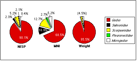
Figure 5.4: Identified fish remains from all analyzed samples, by Number of Individual Specimens, Minimum Number of Individuals, and Bone Weight. All measures adjusted for excavation volume.
Gadus bones also tend to occur in distinct concentrations (Figure 5.5a–c). They are especially concentrated in sample 4/14, an unsurprising result given the discretionary nature of my sample selection process. I had targeted this unit precisely because it contained a preponderance of fish bone of an apparently uniform variety, and because the excavation level intersected with the fish bone midden deposit, Stratum II-9. Cod remains also predominate in samples 4/6, 4/14, and 4/18. Gadus remains are less dominant in the TU7/7 sample, where they are the most abundant fish by bone weight and NISP, but second to Pacific tomcod in MNI. The relative abundance of Gadus and other fish remains in TU7/7 may be skewed by the small sample size of this sample; if the fish bone sample recovered from TU7/7 were larger, non-Gadus fish might appear even more abundant. Other fish taxa eclipse Gadus in TU4, Level 28. Cod were completely absent from this sample, which contained the remains of a single salmonid and a single scorpaenid.
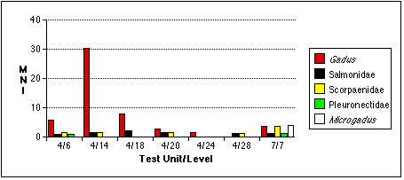
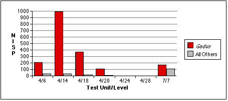
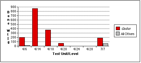
Figure 5.5a–c: Identified fish remains from analyzed samples, by Number of Individual Specimens, Minimum Number of Individuals, and Bone Weight. All measures adjusted for volume.
Distribution of particular Gadus elements in the analyzed faunal collection indicates the differential deposition of cod heads and bodies. In the total sample of identified Gadus individuals, the ratio of MNI computed using the most abundant cranial element (the basioccipital) versus the MNI computed using the most abundant postcranial element (precaudal vertebrae) is 33:3.7, or 8.9 times more cranial than postcranial individuals (Figure 5.6). These figures assume an average of 52.3 vertebrae per individual (Hart 1973:223). While some vertebrae may have been damaged or lost during excavation, the prevalance of fragile cranial elements (18 frontals, for example), suggests that this ratio represented the differential treatment of cod heads.
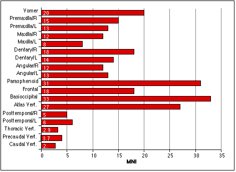
Figure 5.6: Minimum number of Gadus macrocephalus individuals indicated by selected elements, from all analyzed units. Not adjusted for excavation volume.
Three elements appear to vary from the skewed distribution of cranial and postcranial elements: left and right posttemporals and the atlas vertebra. In gadids, pectoral girdle bones such as the posttemporal actually lie posterior to the base of the head (as indicated by the articular surface of the basioccipital; Cannon 1987:45), so I consider these bones marginal to the cranium. When I compute postcranial MNI using left posttemporals (potentially the most abundant postcranial element), this lowers the cranial to postcranial MNI ratio to 33:6, or 5.5. The anomalous distribution of atlas vertebrae is best explained by noting that atlases are the first vertebrae immediate posterior to the basioccipital; each Gadus has only one atlas vertebrae (Cannon 1987). If the distribution of cranial and postcranial elements in the analyzed samples is related to a butchering practice involving the beheading of cod, then I would expect that the atlas would represent the most abundant vertebral element, and a better indicator of cranial MNI than postcranial MNI.
I did not observe the differential distribution of Gadus macrocephalus heads and bodies equally through all sample units, however (Figure 5.7). When adjusted for excavation volume, sample 4/14 has the highest ratio of cranial to postcranial elements: 30.4 individuals computed using the most abundant cranial element versus 4.8 computed using vertebral elements, or 6.3 times more cod heads than cod bodies. Conversely, sample 7/7 has nearly equal distributions of cranial and postcranial elements: at least 3.75 crania and 2.5 vertebral columns, or only 1.5 times more cod heads than cod bodies.
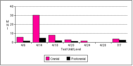
Figure 5.7: Distribution of Gadus macrocephalus by MNI indicated by cranial and postcranial elements. Adjusted for excavation volume.
Finally, the presence of 150 Clupea bones (149 vertebrae and one basioccipital) in the 4/18 sample raised the possibility that herring may also have figured prominently in the Nash Harbor economy. Unfortunately, the field use of 1/4"screens precludes my ability to quantify the importance of these small fish to the Nash Harbor people. I can only note that I missed some amount of herring bones during excavation, and leave the question of their significance open.
Distribution of Mammal Remains
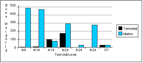
Examination of the mammalian remains from the analyzed samples reveals a wide variety of mammals exploited by Nash Harbor people. The bulk of mammal remains, however, belong to marine animals—pinnipeds and cetaceans. After adjustments for excavation volumes, marine mammals comprise 65.5% of all identified mammal specimens, 70.2% of the identified individuals, and 84.5% of the total bone weight (Figure 5.8).
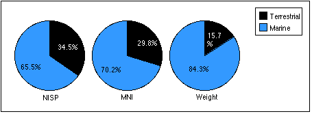
Figure 5.8: Identified terrestrial and marine mammal remains from all analyzed samples, by Number of Individual Specimens, Minimum Number of Individuals, and Bone Weight. All measures adjusted for volume.
With the exception of the TU7, Level 7 sample, marine mammal remains outnumber terrestrial remains in all units by most measures(Figures 5.9 a–c). Land mammal remains outweigh marine mammal remains in the TU4, Level 18 sample, probably because much of the marine mammal material recovered from this level belonged to a small juvenile phocid.
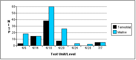
Figures 5.9 a–c: Identified terrestrial and marine mammal remains from analyzed samples, by Number of Individual Specimens, Minimum Number of Individuals, and Bone Weight. All measures adjusted for volume.
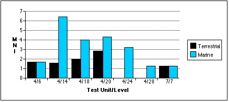
Two groups comprised nearly the entire analyzed terrestrial mammal sample: Canidae and Rangifer. By all measures, canids—including dogs, wolves, and foxes—outnumber Rangifer, although their degree of dominance varies by measure (Figure 5.10). The relative abundance of either genus varies between units and according to the method of measurement, but Canidae remains appear in four sample units, whereas Rangifer remains appear in only three sample units (Figure 5.11 a–c).
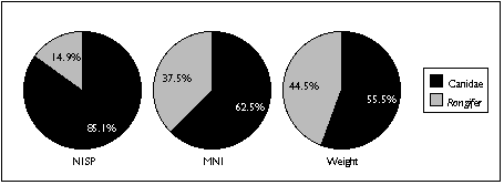
Figure 5.10: Identified Canidae and Rangifer remains from all analyzed samples, by Number of Individual Specimens, Minimum Number of Individuals, and Bone Weight. All measures adjusted for volume.
The difficulty of distinguishing dog species archaeologically complicates interpretation of the canid remains. Four varieties of canid are known to be found on Nunivak Island: domestic dog, wolf, and two species of fox (Lantis 1946). I distinguished between these species in my sample mainly by size. Wolves probably contributed the largest identified canid specimens, found in the TU4/20 sample; foxes probably contributed the smallest—several teeth found in TU4/6. I assumed that other canid remains probably belonged to the domestic dog.
Similary, Rangifer remains could either belong to caribou or reindeer. Caribou populations fluctuated widely on Nunivak Island, and mainland Yupiit armed with high-power rifles exterminated these animals in the late 19th century. Reindeer were introduced by American traders early in the 20th century to replace the extinct caribou (Griffin 1996). The distinction between these two species therefore serves as an important temporal marker—but without Rangifer in the comparative collection, I was unable to distinguish between them. Based on radiocarbon dates and a lack of associated historic artifacts, however, I assumed that all Rangifer remains predate the 20th century, and belong to caribou.
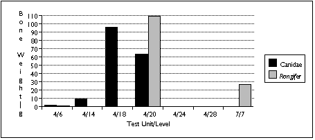
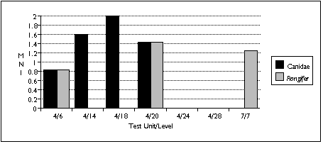
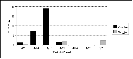
Figure 5.11 a–c: Identified Canidae and Rangifer remains from analyzed samples, by Number of Individual Specimens, Minimum Number of Individuals, and Bone Weight. All measures adjusted for excavation volume.
The relative abundances of sea mammal remains are more difficult to gauge than those of land mammals. Among all samples (adjusted for excavation volumes), Odobenus rosmarus and Phocidae appear to represent the first and second most abundant taxa (Figure 5.12). Phocids contribute 79.6% of the identified specimens, but only 20.1% of the identified bone mass. Odobenids have the opposite distribution, comprising 13.1% of the identified specimens but 57.6% of the identified bone weight. I find this result unsurprising, considering the overall size of each animal—except for beluga, walrus were the most massive animal traditionally taken by the Nunivarrmiut. A few Odobenus specimens would outweigh dozens of phocid bones. In the analyzed Nash Harbor sample, at least two phocid individuals were juveniles. Similarly, Otariidae and Cetacea remains constitute the third and fourth most abundant taxa by all measures.
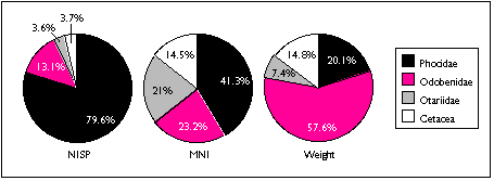
Figure 5.12: Identified marine mammal remains from all analyzed samples, by NISP, MNI, and Bone weight in grams. Adjusted for volume.
Limited sample size and area of excavation may explain the lack of strong patterning in the distribution of marine mammal remains (Figure 5.13 a–c). Phocid remains are the most widely distributed, found in five units. Phocids were also the most concentrated: after adjusting for excavated volume, TU4/18 contained 60 phocid specimens and four individuals. Odobenid remains were also spread throughout the sample, with remains found in four sample units. However, I characterize the sea mammal sample as patchily distributed, and add the caveat that this may reflect sample size rather than a particular Ellikarrmiut hunting or processing pattern.
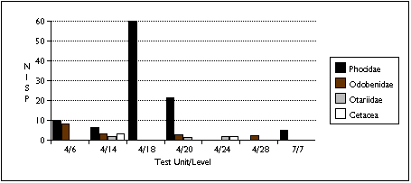
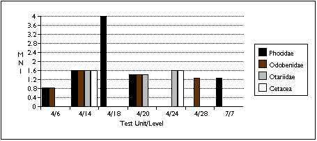
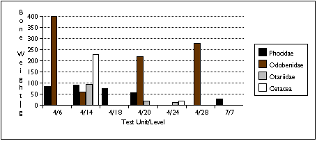
Figure 5.13 a–c: Identified marine mammal remains from analyzed samples, by NISP, MNI, and Bone Weight ingrams. All measures adjusted for volume.
Distribution of Invertebrate Remains
Mytilus remains dominate the analyzed invertebrate sample (Figure 5.14). When adjusted for variations in excavation volume, Mytilus constitute 89.2% of the all invertebrate remains. Macoma shell contribute 9.9% of the shell sample, with less than 1% of the shell sample deriving from Balanus (acorn barnacle) and unidentified marine gastropods.
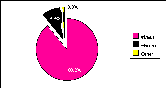
Figure 5.14: Identified invertebrate remains from all analyzed samples, by shell weight.
Adjusted for excavation volume.
Virtually all shellfish remains were found in the TU7/7 sample; this certainly reflected a bias in sample selection as well as the actual distribution of shellfish (Figure 5.15). TU7 contained the largest concentration of shell midden material discovered by archaeologists at Nash Harbor, and I included one sample from TU7 to provide some data on invertebrate harvesting patterns. I also noted a large amount of Mytilus shell in the fish bone midden deposit intersecting TU4/14, and I identified several Macoma shell fragments in the TU4/6 sample.
The analysis of invertebrates almost certainly under-represents their actual abundance at Nash Harbor. Screeners noted amounts of Mytilus periostraca during excavation; many of these remains were crushed during screening, or blown out of the screens by the strong Nunivak winds. The use of 1/4" screens during excavation also led to the loss of an unknown amount of shell, which was often so finely fragmented that it passed through the excavation screens.
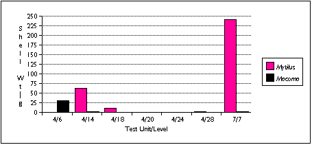
Figure 5.15: Distribution of invertebrate remains by shell weight, adjusted for excavation volumes.
Distribution of Major Taxonomic Groups
After adjusting measures for excavation volumes, fish are probably the most abundant animals, representing 85.2% of the identified vertebrate specimens, 44.6% of the identfied vertebrate individuals, and 41.7% of the total weight of the analyzed sample (Figure 5.16). Mammals contribute 46.2% of the total weight of the analyzed sample, but only 18.3% of identified vertebrates, and 8.2% of vertebrate specimens. Conversely, birds represent 37% of the identified vertebrate individuals, but only about 8% of either individual vertebrate specimens or total faunal weight. Shellfish, because of their highly fragmentary remains, are comparable to vertebrates only in shell weight, where they constitute a scant 3.7% of the analyzed remains.
Variations in the size of the different taxa partly explain these contradictory data. Except for Mustelidae, the smallest mammal individual would outweigh the largest individual of any other taxon. The remains of a single walrus individual, represented only by a few fragments, outweighs dozens of more complete bird skeletons. Bird bones, on the other hand, were less fragmented than mammal bones, and easier to identify generally. While I could identify 68.5% of the bird specimens, I could only identify 55.1% of the mammal specimens. Thus, the MNI for birds would necessarily be higher than for other taxa.
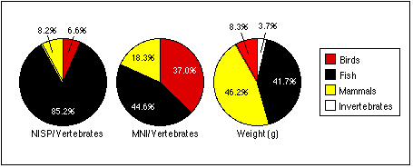
Figure 5.16: Identified animal remains from all analyzed samples, by Number of Individual Specimens, Minimum Number of Individuals, and Bone Weight. Measures for NISP and weight include identified and unidentifed remains; all measures adjusted for excavation volume.
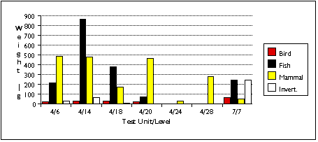
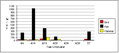
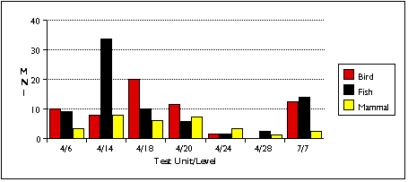
Figure 5.17 a–c: Distribution of faunal remains in analyzed units, by Bone Weight in grams, NISP, and MNI. All measures adjusted for volume. Includes identified and unidentified remains.
Fish bones had the widest spatial distribution of any taxa but also tended to occur in the largest concentrations—outranking other taxa by all measures in TU4/6 and TU7/7 (Figure 5.17 a–c) . Bird remains tended to be widely distributed, but not as concentrated, except as measured by MNI in TU4/18. Mammal remains were found in all samples, in varying quantities, again probably as a function of animal and sample size. Only mammal remains were found in any measurable abundance in TU4/24 and TU4/28. Invertebrate remains were the least highly dispersed of all taxa, found in significant quantities only in TU7/7, with a very few found in TU4/6 and TU4/14.
After careful consideration of the spatial distribution of faunal remains, I can characterize the analyzed samples with the following summary statements:
No taxon predominated in TU4/6, except that Gadus—as in other units where fish were found in significant quantities—were clearly the most abundant fish. Except for a few Macoma, invertebrate remains were generally scarce. The mammalian sample was typified by a few large Odobenus specimens.
TU4/14 represented a trash heap of fish bones, associated with a processing activity resulting in the differential deposition of Gadus crania here. Remains of other taxa, especially gulls, cliff birds, and sea mammals, were also abundant.
TU4/18 represented a deposit of fish and bird bones. As with TU4/14, Gadus crania were more numerous than vertebrae. Cliff birds' remains were most concentrated in this sample. Seal and canid predominated among mammalian remains, although a few fragments of whale bone made Cetacea more abundant by bone weight. The presence of Clupea harengus vertebrae in the bulk sample from TU4/18 suggests that herring may also be abundant in this unit, but I can not estimate their relative abundance.
Faunal materials were more scarce in TU4/20 than in the analyzed samples above it. A few Odobenus specimens outweighed all other animal remains, but Phocidae were the most common sea mammals by NISP. Cliff birds remained the most common avians.
Faunal materials were almost entirely lacking in TU4/24 and TU4/28, except for a few large Odobenus specimens in TU4/28. Notably, these units contained no Gadus remains. The paucity of trash in these levels may bolster the hypothesis that this stratum represented a collapsed structure, as advanced in Section 2.
Mytilus remains predominated in TU7/7, almost exceeding fish remains in weight. Gadus remains were common, but unlike other samples containing Gadus, cranial and postcranial individuals were nearly equally represented. Quite a few cliff birds were found here as well. I characterize TU7/7 as associated with shellfish and cliff bird processing.